

Demystifying the Transformer: How AI Learned to Understand Context


Try typing “Why is the sky” into your phone. Before you finish, it guesses “blue” as the next word.
How did it know? The phone does not actually understand the meaning of your sentence, but it does know which word is most likely to come next.
In the early 1990s, video games started to display a type of artificial intelligence. I spent a lot of quarters on Street Fighter II and Mortal Kombat. When you fought the computer, it felt like playing a real person. It blocked your punches and knew what combos to use to win the fight. That was a big jump from old-school Galaga, where the aliens swooped in the same pattern every time.
The trick was that the computer knew your move the millisecond you hit the button, allowing it to choose the proper counter move. It was a mere illusion that fooled us. Then, in the 2010s, machine learning took off. ChatGPT followed in late 2022, and AI has been the most talked-about topic ever since.
At the heart of ChatGPT is an invention called the transformer. This is the story of how it was built, one step at a time, with the math picked apart along the way.
Computers only speak numbers
Every computer is made of billions of tiny switches. Each one is either on (1) or off (0). A computer doesn’t understand words or feelings. It only understands numbers.
So how do you translate words into numbers that a computer can actually understand? That’s the big question this story answers.
Phase 1: Count every word in your file
This all began with the bag of words in the 1950s. Much like it sounds, you take every word in a document or corpus and count them. The order, meaning and grammar don’t matter. This is simply a word count. If the most common words in an article are “Chicago,” “Bears” and “football,” you could assume the article was about a recent Bears game.
To create a little more meaning, developers usually remove the stop words. These are words like “the” and “is” that are fairly common but have no real meaning. Then you go through a process called stemming. Just like trimming a rose bush, we shorten words to just their root. A word like “running” turns into “run.”
Here is the basic formula behind this process.
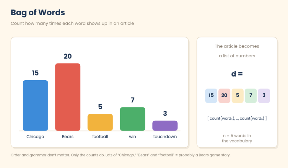
d = [ count(word₁), count(word₂), … , count(wordₙ) ]
• d is the document. This ultimately creates an array of numbers known as a vector.
• count(word) is how many times that word shows up.
• n is how many different words are in our vocabulary.
Here’s what that looks like for two tiny sentences:
“Motorola created the first handheld cell phone in Chicago.” → motorola: 1, create: 1, first: 1, handheld: 1, cell: 1, phone: 1, chicago: 1
“The Chicago Cubs won the World Series in 2016.” → chicago: 1, cub: 1, won: 1, world: 1, series: 1, 2016: 1
That’s great for simple search. If you are looking for information about Chicago, it would likely be in an article where “Chicago” has a high word count.
But there’s a catch. The only word these two sentences share is “Chicago,” so the computer thinks they’re related, even though one is about phones and the other is about baseball. In reality, the two topics have nothing to do with each other. A bag of words can count, but it can’t understand relationships.
Phase 2: Word2Vec gives every word a location
In 2013, a Google team led by Tomas Mikolov released Word2Vec. This phase moved from just counting words to placing them on a map using vectors. In other words, words with similar meanings get similar patterns of numbers.
“Bears” and “Cubs” both show up near words like “game,” “season” and “score.” “Italian beef” shows up near “sandwich” and “giardiniera.” So Word2Vec gives every word a location on a giant map.
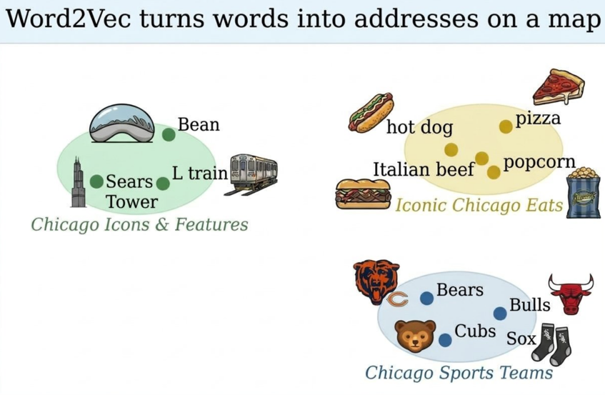
Words that show up in similar places end up close together. Chicago’s teams live in one neighborhood and its food in another. But notice that every word gets just one spot on the map.
How close are two words?
If you look at which words show up near each other across millions of articles, you start to see the same groups of words appear by topic. To compare two words, you multiply their matching numbers and add them up. This is the dot product:
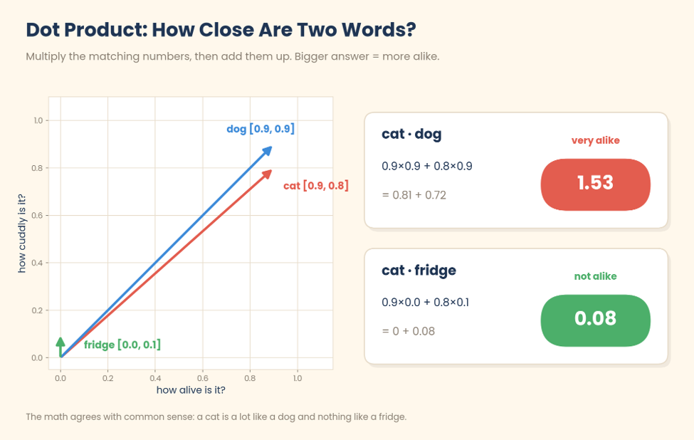
a · b = a₁×b₁ + a₂×b₂ + … + aₙ×bₙ
• a and b are the number lists for two words.
• a₁ is the first number in a, a₂ is the second, and so on.
• A bigger answer means the words are more alike.
Let’s try a made-up map with just two numbers per word: “how alive is it?” and “how cuddly is it?”
• cat = [0.9, 0.8] dog = [0.9, 0.9] fridge = [0.0, 0.1]
• cat · dog = 0.81 + 0.72 = 1.53
• cat · fridge = 0 + 0.08 = 0.08
Cat and dog score high. Cat and fridge score almost nothing. The math agrees with common sense.
The word math trick
Now that everything has been mapped, you can actually add and subtract values and get new results. The step from “baseball” to “Cubs” is the same as the step from “football” to “Bears.” That is why this formula works:
Bears – football + baseball = Cubs
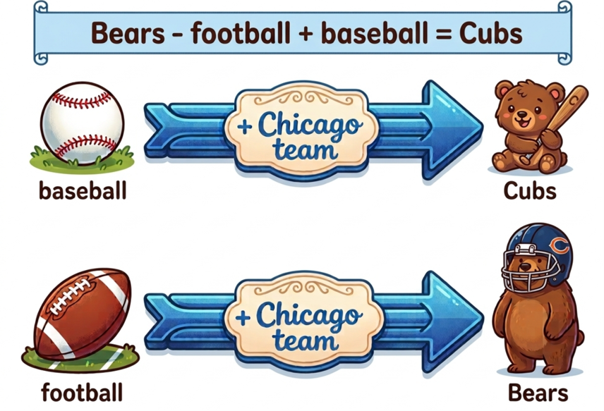
The arrow from baseball to Cubs matches the arrow from football to Bears.
Guessing the missing word
So how did researchers actually get this to work? First, they built a simple neural network that scores how likely each word is to fit in a blank. Then they let the computer learn by playing a guessing game billions of times. Hide a word in a sentence like “Chicago is known for deep-dish ___.” Then have the computer guess it.
The computer could guess anything from “mouse” to “lasagna” to “pizza.” Ultimately, the one with the highest probability should be “pizza.” Then it turns the scores into chances with a formula called softmax.
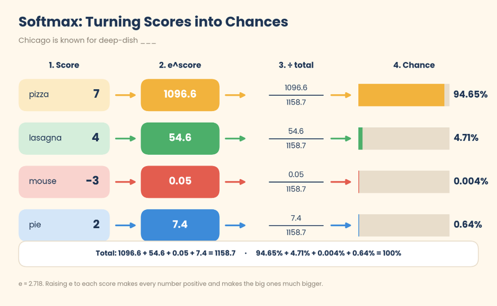
P(wordᵢ) = esᵢ ÷ ( es₁ + es₂ + … + esᵥ )
• sᵢ is the score for word number i.
• e is a special number, about 2.718. Raising it to a power makes every score positive and makes big scores stand out.
• V is the number of words in the vocabulary.
• P(wordᵢ) is the chance that word i is the answer. All the chances add up to 100%.
In this scenario, I would expect pizza to score about 95%. Lasagna may be about 5%, and I hope mouse would be nearly zero.
Now for the part that makes all modern AI work. When the computer guesses wrong, it gets a loss score that measures how wrong it was. Then it traces its steps back through a process called backpropagation to figure out why. Over time, the score improves, almost like playing “hotter or colder.” Each wrong guess tells the computer which direction to move.
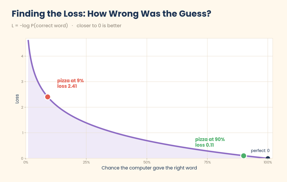
L = −log P(correct word)
• log here means the natural log. For a chance between 0 and 1, it gives a negative number. The minus sign flips it positive.
• If the answer was “pizza” and the computer scored it at 90%, the loss is about 0.11. If it gave pizza only 9%, the loss jumps to 2.41.
The closer the loss is to 0, the better. Zero represents a perfect answer.
The computer improves by comparing each guess to the actual answer. Backpropagation works out how much each part of the model contributed to the mistake. Every number on the map is like a little knob, called a weight. After each guess, it turns every knob a tiny bit in the direction that lowers the loss. As the guesses get better, the loss is reduced. This is gradient descent:
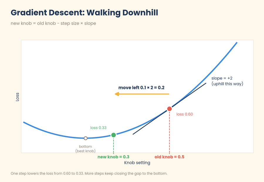
new knob = old knob − step size × slope
• slope tells you which way is uphill. Subtracting it moves the knob the opposite way, downhill, where the loss gets smaller.
• step size is how far you move each time. Too big and you overshoot. Too small and it takes forever.
• Example: if the knob is at 0.5, the slope is 2 and the step size is 0.1, the new knob is 0.5 − 0.1 × 2 = 0.3.
Think about playing Super Mario Bros. blindfolded. The first few times, you would die quickly. If you did this a billion times, you could time all your jumps, find all the power-ups and discover all the warp zones.
The best part is that nobody has to label anything. This is known as self-supervised learning, because the text supplies its own answer key. You just hide a word and check the guess. This laid the groundwork for today’s chatbots.
Phase 3: One word at a time is too slow
Word2Vec was a huge step in the right direction, but it had a blind spot. It could not comprehend words with more than one meaning.
Think about the word “pop.” In “I heard a huge pop,” it’s a loud, sudden noise. In “Grab me a pop from the refrigerator,” it’s a beverage or soda. Word2Vec gave both the same vector because it doesn’t understand context. To fix that, the computer has to read the words around it.
So researchers turned to recurrent neural networks, or RNNs. They read a sentence one word at a time, keeping a small, running memory as they go.
However, this small memory made RNNs forgetful, and reading one word at a time was slow. You can’t read word 10 until you’ve finished word 9, so the work can’t be split up and run in parallel.
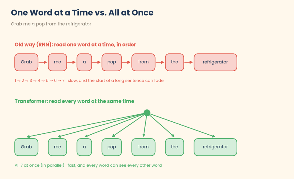
RNNs read in a line. Transformers read the whole sentence at once.
In 2014, researchers found a clever patch. The network could look back at every earlier word and pick the most relevant ones. This is called attention.
Phase 4: “Attention Is All You Need”
In June 2017, eight Google researchers published a paper with that exact title. It was truly revolutionary and gave us the first transformer.
A transformer reads every word at the same time and lets each word decide which other words matter to it.
Because it reads every word at once, a transformer can split its work across thousands of GPUs, which sped up training dramatically. To keep “Bears beat the Packers” and “Packers beat the Bears” straight, each word is also indexed with its place in line.
How self-attention works
Self-attention lets the computer read each word while comparing it to all the other words in the sentence. Imagine you’re standing on the shore of Lake Michigan on a foggy night, next to a lighthouse. The lighthouse is the word “bank” in “We fished from the river bank.” The other words are out on the water at different distances. “River” is just 4 feet away. “Fished” is 30 feet out. “We,” “from” and “the” are far off near the horizon. When the lighthouse sweeps its beam across the water, the closest words light up bright and clear, and the distant ones barely show through the fog. That’s attention. The closer a word is to “bank” in meaning, the brighter it shines. “River” is closest because it scores highest when compared with “bank,” a match the model learned from reading millions of sentences. If “money” or “loan” had been in the sentence, they would have been right next to the lighthouse instead, and “bank” would mean something completely different.

The closer the word, the brighter it shines. “River” matters most to “bank.”
These are the three pieces that make self-attention work:
• A query (Q): the question it asks, like “What am I looking for?”
• A key (K): a name tag that says, “Here’s what I’m about.”
• A value (V): the information it shares if it gets picked.
It’s like a library. Your query is what you type into the search box. Keys are the titles on the book spines. Values are what’s inside the books.
Here’s the most important formula in this whole story:
Attention(Q, K, V) = softmax( Q·KT ÷ √dₖ ) · V
Let’s break this down into four steps.
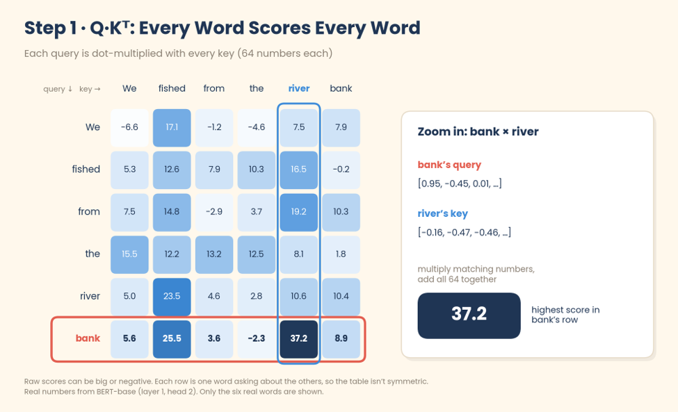
1. Q·KT: Compare every question with every name tag using dot products, just like cat · dog. High score means “you matter to me.”
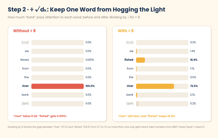
2. ÷ √dₖ: Shrink the scores a bit so no single word hogs all the attention.
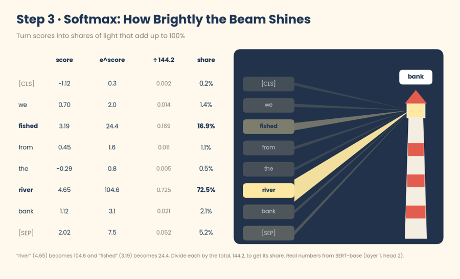
3. softmax: Turn the scores into percentages, which set how brightly the beam lights up each word.
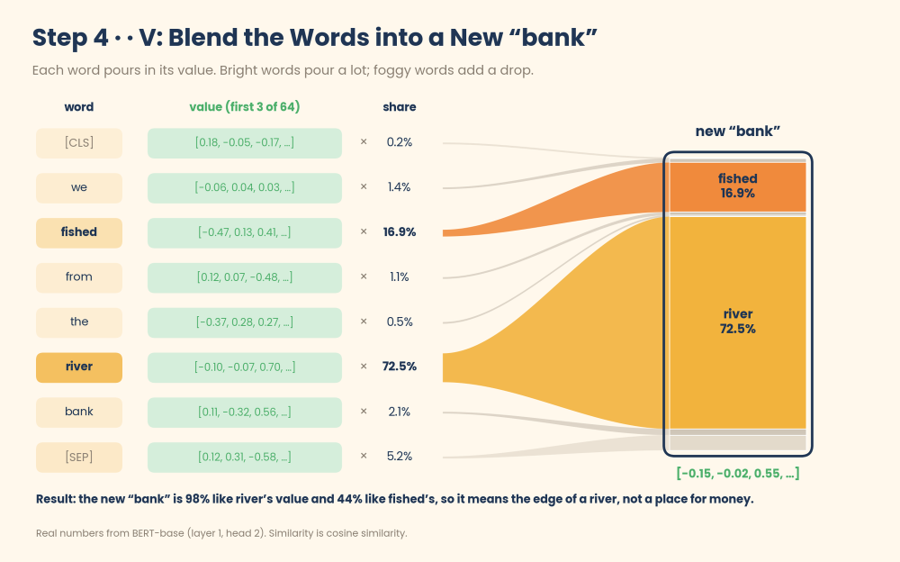
4. · V: Blend the words’ information using those percentages. Brightly lit words count a lot. Words lost in the fog barely count.
Notice how it reuses the dot product and softmax from Word2Vec.
A quick note for math fans
To keep things simple, I’ve described attention as one word comparing itself to one other word at a time. Real transformers stack every word’s query into one big table of numbers, called a matrix, and every word’s key into another. Multiplying the two tables does every word-to-word dot product in a single step. That’s what Q·KT really means.
In big models, those tables have thousands of rows and columns, and this happens in every layer. That’s exactly the kind of math GPUs are built to do fast.
A transformer does this with several lighthouses at once, each sweeping its own beam. One might track who’s doing the action. Another might link “it” back to the right noun. Then it stacks the whole process in layers, like reading the sentence six times and understanding it a little better each time.
Phase 5: GPT and BERT
More improvements came in 2018, when two famous models put the transformer to work in opposite ways.
First, GPT (from OpenAI) introduced dynamic generation. This new process writes brand-new sentences on the fly by predicting one word at a time.
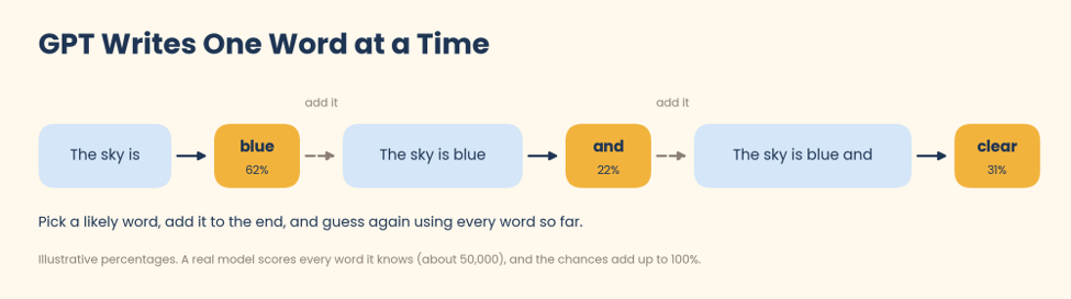
P( next word | all the words so far )
• The | sign means “given.” So this reads, “the chance of the next word, given everything before it.”
• Softmax turns the transformer’s scores into those chances, just like in the guessing game.
GPT picks a likely word, adds it to the end, and guesses again. Softmax helps it find the most likely next word each time. It does this word by word until it completes a sentence or paragraph. That’s the same idea behind your phone suggesting “blue” when you type “The sky is.” If you changed the sentence to start with “The Martian sky is,” it would choose “red” or “brown” instead.
Later that same year, BERT (from Google) arrived. It plays the same fill-in-the-blank game as Word2Vec, but it hides random words anywhere in a sentence and uses the whole sentence, before and after the blank, to guess them. Researchers trained it on all of English Wikipedia plus a collection of about 11,000 unpublished books called BookCorpus. The computer learned to fill in the blanks like a Mad Libs puzzle. It also learned to tell whether one sentence naturally follows another.
Models built on BERT often use a trick called sentence-level pooling. When you read a long sentence, you don’t memorize every word. You remember the point. Pooling does the same thing, creating one vector for an entire sentence instead of one per word. That idea paved the way for vector databases and retrieval-augmented generation (RAG).
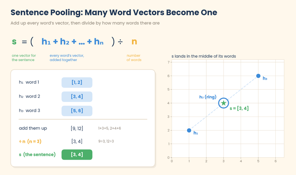
s = ( h₁ + h₂ + … + hₙ ) ÷ n
• h₁ … hₙ are the final vectors for each of the n words.
• s is one vector that stands for the whole sentence.
• Example: [1, 2], [3, 4] and [5, 6] average to [3, 4].
Researchers also tested BERT on SQuAD, the Stanford Question Answering Dataset, where a model reads a passage and has to find the answer to a question inside it.
Phase 6: Increasing model and parameter size
After 2018, the recipe barely changed, but the overall size of the model increased drastically.
• GPT-2 (2019) had 1.5 billion parameters (or knobs) and wrote smooth paragraphs.
• GPT-3 (2020) had 175 billion parameters and could write essays, poems and code.
• ChatGPT (November 2022) added training where people rated its answers, so it learned to be helpful and conversational.
Under the hood, it was the same guessing game, the same softmax and the same lighthouse beams, just a lot more of them running a lot faster with larger, better-trained models.
Putting it all together
When I fought the computer in Mortal Kombat, it felt like a person was on the other side of the screen. That was just an illusion designed by developers who anticipated common patterns.
Today’s AI can feel that way too. While there’s no human being on the other side, it’s still just as remarkable. As this article shows, it was all built on a chain of ever-evolving ideas about patterns and word probabilities. Here’s the short version:
1. Counting words turned text into numbers.
2. Word2Vec gave those numbers meaning.
3. RNNs taught computers that order matters.
4. Attention let every word look at every other word at once.
5. Scale turned a research idea into something you can chat with.
It isn’t magic. It’s a sophisticated chain of probabilities. At the end of the day, these are statistical models that use multiplying, adding and probabilities to guess a result, grade it and then try again billions of times until they get good at it.
So the next time your phone finishes your sentence with “blue,” you’ll know what happened. A few thousand tiny lighthouses swept through the fog, lit up the words that mattered and helped the computer make its best guess. And if you ever type “Chicago is known for deep-dish,” I’m betting it guesses pizza.


Comments